

donsutherland1
-
Posts
24,154 -
Joined
Content Type
Profiles
Blogs
Forums
American Weather
Media Demo
Store
Gallery
Everything posted by donsutherland1
-
A sustained period of above to much above normal temperatures is now developing. Tomorrow will again be fair and mild. In general, above normal temperatures will persist through the end of March. There is potential for near record to record warm conditions to occur in eastern Canada on Monday and Tuesday. The ENSO Region 1+2 anomaly was +0.9°C and the Region 3.4 anomaly was -0.3°C for the week centered around March 10. For the past six weeks, the ENSO Region 1+2 anomaly has averaged -0.20°C and the ENSO Region 3.4 anomaly has averaged -0.80°C. La Niña conditions will likely give way to neutral-cool ENSO conditions as the spring progresses. The SOI was +5.79 today. The preliminary Arctic Oscillation (AO) figure was +1.469 today. The 31° temperature recorded at Central Park on March 19 could be New York City's last freeze of 2020-21 based on a combination of the latest ensemble guidance and the diminishing frequency of April freezes. April freezes have become less frequent in recent years. During the 1991-2020 base period, there were 12 cases where the last freeze occurred in April. The last time the temperature fell to freezing in April occurred in 2018. Select April Statistics: 1951-80: Years with freezes: 17; Mean days with lows of 32° or below: 1.1 1961-90: Years with freezes: 17; Mean days with lows of 32° or below: 1.3 1971-00: Years with freezes: 16; Mean days with lows of 32° or below: 1.2 1981-10: Years with freezes: 12; Mean days with lows of 32° or below: 1.0 1991-20: Years with freezes: 12; Mean days with lows of 32° or below: 1.0 Least years with freezes: 10, 1984-2013 Most years with freezes: 26, 1874-1903, 1880-1909, 1895-1924, 1896-1925, and 1897-1926 Lowest number of average days with temperatures of 32° or below: 0.8, 1983-2012, 1984-2013, 1985-2014, and 1986-2015 Highest number of average days with temperatures of 32° or below: 3.7, 1871-1900 and 1872-1901 Least days in April with temperatures of 32°: 0, Most Recent: 2020 Least days in April with temperatures of 32°: 11, Most Recent: 1874 Based on sensitivity analysis applied to the latest guidance, there is an implied 87% probability that New York City will have a warmer than normal March. March will likely finish with a mean temperature near 44.4° (1.9° above normal).
-
Morning thoughts... The low temperature at Central Park was 33° this morning. As a result, yesterday’s 31° figure was likely New York City’s last freeze of 2020-21, based both on the latest ensemble guidance and diminishing frequency of April freezes. Under bright sunshine, today will feature a springlike afternoon. High temperatures will reach the middle and upper 50s in most of the region. Likely high temperatures around the region include: New York City (Central Park): 57° Newark: 59° Philadelphia: 59° Tomorrow will be continued fair and mild.
-
Earlier today, the temperature fell to 31° in New York City. Overnight, the temperature could again approach or reach freezing in Central Park. Afterward, it is possible that New York City will not see the temperature fall to freezing until some time next fall, as the remainder of March will likely see above freezing temperatures. April freezes have become less frequent in recent years. During the 1991-2020 base period, there were 12 cases where the last freeze occurred in April. The last time the temperature fell to freezing in April occurred in 2018. Select April Statistics: 1951-80: Years with freezes: 17; Mean days with lows of 32° or below: 1.1 1961-90: Years with freezes: 17; Mean days with lows of 32° or below: 1.3 1971-00: Years with freezes: 16; Mean days with lows of 32° or below: 1.2 1981-10: Years with freezes: 12; Mean days with lows of 32° or below: 1.0 1991-20: Years with freezes: 12; Mean days with lows of 32° or below: 1.0 Least years with freezes: 10, 1984-2013 Most years with freezes: 26, 1874-1903, 1880-1909, 1895-1924, 1896-1925, and 1897-1926 Lowest number of average days with temperatures of 32° or below: 0.8, 1983-2012, 1984-2013, 1985-2014, and 1986-2015 Highest number of average days with temperatures of 32° or below: 3.7, 1871-1900 and 1872-1901 Least days in April with temperatures of 32°: 0, Most Recent: 2020 Least days in April with temperatures of 32°: 11, Most Recent: 1874 The coming weekend will mark the start of a warming trend. Since 1950, nearly 60% of days two weeks after the AO reached +3.000 or above in the March 1-15 period were warmer than when the AO reached +3.000 or above. The AO reached +3.000 on March 10. The mean increase was 2.8°. This suggests that it is more likely than not that the closing week of March could see a return to warmer conditions. Most of the guidance favors the development of warmer conditions that would continue through the remainder of the month. There is potential for near record to record warm conditions to occur in eastern Canada early next week. The ENSO Region 1+2 anomaly was +0.9°C and the Region 3.4 anomaly was -0.3°C for the week centered around March 10. For the past six weeks, the ENSO Region 1+2 anomaly has averaged -0.20°C and the ENSO Region 3.4 anomaly has averaged -0.80°C. La Niña conditions will likely give way to neutral-cool ENSO conditions as the spring progresses. The SOI was -2.20 today. The preliminary Arctic Oscillation (AO) figure was +0.238 today. Based on sensitivity analysis applied to the latest guidance, there is an implied 85% probability that New York City will have a warmer than normal March. March will likely finish with a mean temperature near 44.3° (1.8° above normal).
-
Morning thoughts... Following a departing storm that ended with a little light snow in the New York City region, today will be partly cloudy and windy. It will be unseasonably chilly. High temperatures will reach the lower and middle 40s in most of the region. Likely high temperatures around the region include: New York City (Central Park): 44° Newark: 45° Philadelphia: 47° A pronounced warming trend will likely commence during the weekend. As a result, should the temperature fall to freezing tomorrow morning, there is a chance that it could be Central Park’s last freeze of the 2020-21 season. Early next week could see near record to record warmth in parts of eastern Canada. Finally, it is likely that Central Park will fall short of receiving the 1.4” snow needed to reach 40.0” for winter 2020-21. Since 1869, there were 30 cases that saw no measurable snowfall during March 1-19. Mean snowfall for the remainder of the snow season came to 0.8”. 60% of cases saw no measurable snowfall, 77% of cases saw less than 1” of snow, 23% saw 1” or more snow, and 17% saw 2” or more snow during the remainder of the snow season. The most snowfall from such cases was 5.0” during 1998. The most recent such case occurred in 2020 when no measurable snow was reported after March 19.
-
Colder air will press southward tonight. As the temperature falls, rain will change to snow in parts of the Northeast. Precipitation will likely total 0.50" - 1.50" from Philadelphia to Boston with some higher amounts. There could still be an area of 1"-3" snowfall with some locally higher amounts in an area running through New England, that could include Boston and/or Worcester. There is a chance that the rain could end as a period of snow or flurries even in New York City and its nearby suburbs. The coming weekend will likely mark the start of a warming trend. Since 1950, nearly 60% of days two weeks after the AO reached +3.000 or above in the March 1-15 period were warmer than when the AO reached +3.000 or above. The AO reached +3.000 on March 10. The mean increase was 2.8°. This suggests that it is more likely than not that the closing week of March could see a return to warmer conditions. Most of the guidance favors the development of warmer conditions that would continue through the remainder of the month. The ENSO Region 1+2 anomaly was +0.9°C and the Region 3.4 anomaly was -0.3°C for the week centered around March 10. For the past six weeks, the ENSO Region 1+2 anomaly has averaged -0.20°C and the ENSO Region 3.4 anomaly has averaged -0.80°C. La Niña conditions will likely give way to neutral-cool ENSO conditions as the spring progresses. The SOI was -2.49 today. The preliminary Arctic Oscillation (AO) figure was -0.117 today. On March 17 the MJO data was unavailable. MJO data will no longer be posted until the data is again available. The significant December 16-17 snowstorm during what has been a blocky December suggests that seasonal snowfall prospects have increased especially from north of Philadelphia into southern New England. At New York City, there is a high probability based on historic cases that an additional 20" or more snow will accumulate after December. Since January 1, New York City has picked up 28.1" snow. Winters that saw December receive 10" or more snow, less than 10" in January, and then 10" or more in February in New York City, saw measurable snowfall in March or April in 83% of cases. Winter 2009-2010 was the exception where only a trace of snow was recorded. This group of winters saw 6" or more snow during the March-April period in 50% of the cases. All said, it is more likely than not that there will be measurable snowfall after February. Based on sensitivity analysis applied to the latest guidance, there is an implied 81% probability that New York City will have a warmer than normal March. March will likely finish with a mean temperature near 44.0° (1.5° above normal).
-
It’s too soon for me to make any calls about snowfall for April. I do think this will be the last chance for snowfall in March given the forecast pattern and strong consensus on the guidance about warmer conditions for the remainder of the month beginning Sunday.
-
Morning thoughts... Tornadoes, large hail, and damaging winds pounded parts of the Gulf Region yesterday. Today, the focus of the severe weather will stretch from Georgia, across the Carolinas, and into Virginia before moving offshore. At 7:50 am, an area of rain was advancing into eastern Pennsylvania and southern New Jersey. Rain will develop this morning in most of the region. Precipitation will likely total 0.50”-1.50” from Philadelphia to Boston with some locally higher amounts in excess of 2.00”. High temperatures will reach the upper 40s and lower 50s in most of the region. Likely high temperatures around the region include: New York City (Central Park): 50° Newark: 50° Philadelphia: 52° As colder air presses southward tonight, rain will change to snow across central New York State and central New England. That snow will push southward. There will be an area of 2”-4” snowfall with locally higher amounts in parts of New England, including Boston and Worcester. The rain could end as a period of snow or flurries even in New York City and its nearby suburbs. A pronounced warming trend will likely commence during the weekend. As a result, there is a chance that the coming weekend could see Central Park’s last freeze of the 2020-21 season.
-
Tomorrow will be rainy, as a developing storm moves eastward and then offshore tomorrow night. As colder air pushes in, rain will change to snow in parts of the Northeast. There will likely be an area of 2"-4" snowfall with some local amounts of 6" over in an area running through New England, including Boston and Worcester. There is a chance that the rain could end as a period of snow or flurries even in New York City and its nearby suburbs. The coming weekend will likely mark the start of a warming trend. Since 1950, nearly 60% of days two weeks after the AO reached +3.000 or above in the March 1-15 period were warmer than when the AO reached +3.000 or above. The AO reached +3.000 on March 10. The mean increase was 2.8°. This suggests that it is more likely than not that the closing week of March could see a return to warmer conditions. Most of the guidance favors the development of warmer conditions that would continue through the remainder of the month. The ENSO Region 1+2 anomaly was +0.9°C and the Region 3.4 anomaly was -0.3°C for the week centered around March 10. For the past six weeks, the ENSO Region 1+2 anomaly has averaged -0.20°C and the ENSO Region 3.4 anomaly has averaged -0.80°C. La Niña conditions will likely give way to neutral-cool ENSO conditions as the spring progresses. The SOI was -2.68 today. The preliminary Arctic Oscillation (AO) figure was -0.288 today. The AO's 5-day change from its March 12 peak of +5.656 is -5.994. That is the 4th largest 5-day decline on record. The only higher cases occurred during November 8-13, 1959 (-6.439), January 20-25, 1976 (-6.036), and January 19-24, 1976 (-5.997). Daily recordkeeping began on January 1, 1950. On March 16 the MJO data was unavailable. The significant December 16-17 snowstorm during what has been a blocky December suggests that seasonal snowfall prospects have increased especially from north of Philadelphia into southern New England. At New York City, there is a high probability based on historic cases that an additional 20" or more snow will accumulate after December. Since January 1, New York City has picked up 28.1" snow. Winters that saw December receive 10" or more snow, less than 10" in January, and then 10" or more in February in New York City, saw measurable snowfall in March or April in 83% of cases. Winter 2009-2010 was the exception where only a trace of snow was recorded. This group of winters saw 6" or more snow during the March-April period in 50% of the cases. All said, it is more likely than not that there will be measurable snowfall after February. Based on sensitivity analysis applied to the latest guidance, there is an implied 74% probability that New York City will have a warmer than normal March. March will likely finish with a mean temperature near 43.7° (1.2° above normal).
-
SPC’s day 1 convective outlook:
-
Morning thoughts... Today, the Gulf States will feature a significant outbreak of severe weather. Widespread severe thunderstorms will be likely. Those thunderstorms could bring large hail, damaging winds, and tornados. There is potential for at least one or more EF-3 or above tornados given the extreme CAPE that is forecast in some parts of the Gulf Region. In the northern Middle Atlantic and southern New England regions, quieter weather will prevail. In the wake of yesterday’s weak system that brought flurries to parts of the region, today will be partly to mostly cloudy and milder. High temperatures will reach the upper 40s in most of the region. Likely high temperatures around the region include: New York City (Central Park): 49° Newark: 49° Philadelphia: 52° On Thursday night, a developing nor’easter will move offshore. That storm will bring a swath of 2”-4” snowfall with locally higher amounts to parts of New England, including Boston, Providence, and Worcester. The rain could end as a period of snow or flurries even in New York City and its nearby suburbs. A pronounced warming trend will likely commence during the weekend. As a result, there is a chance that the coming weekend could see Central Park’s last freeze of the 2020-21 season.
-
No problem. A quick video clip from May 9, 2020:
-
A weak system touched off some scattered snow flurries today into this evening. Following the passage of today's weak system, tomorrow will likely see a return to sunshine and milder conditions. Nevertheless, the remainder of the March 16-19 period could still offer some opportunity for at least some snowfall in parts of the region as a developing nor'easter moves offshore Thursday night. There will likely be an area of 2"-4" snowfall with some local amounts of 6" over a part of New England, including Boston, Providence, and Worcester. There is some chance that the rain could end as a period of snow or flurries even in New York City and its nearby suburbs. The coming weekend will likely mark the start of a new warming trend. Since 1950, nearly 60% of days two weeks after the AO reached +3.000 or above in the March 1-15 period were warmer than when the AO reached +3.000 or above. The AO reached +3.000 on March 10. The mean increase was 2.8°. This suggests that it is more likely than not that the closing week of March could see a return to warmer conditions. Most of the guidance favors the development of warmer conditions that would continue through the remainder of the month. Tomorrow could see greatly elevated CAPE in an area extending from eastern Texas across the Gulf States. Extreme CAPE levels are likely over a portion of the Gulf States. As a result, there will be a high probability of severe thunderstorms with hail and possible tornados in parts of that area, especially in the Gulf States. That risk of severe weather will then likely move into the Carolinas and Virginia on Thursday and then offshore afterward. The ENSO Region 1+2 anomaly was +0.9°C and the Region 3.4 anomaly was -0.3°C for the week centered around March 10. For the past six weeks, the ENSO Region 1+2 anomaly has averaged -0.20°C and the ENSO Region 3.4 anomaly has averaged -0.80°C. La Niña conditions will likely give way to neutral-cool ENSO conditions as the spring progresses. The SOI was -5.51 today. The preliminary Arctic Oscillation (AO) figure was +0.651 today. On March 15 the MJO data was unavailable. The significant December 16-17 snowstorm during what has been a blocky December suggests that seasonal snowfall prospects have increased especially from north of Philadelphia into southern New England. At New York City, there is a high probability based on historic cases that an additional 20" or more snow will accumulate after December. Since January 1, New York City has picked up 28.1" snow. Winters that saw December receive 10" or more snow, less than 10" in January, and then 10" or more in February in New York City, saw measurable snowfall in March or April in 83% of cases. Winter 2009-2010 was the exception where only a trace of snow was recorded. This group of winters saw 6" or more snow during the March-April period in 50% of the cases. All said, it is more likely than not that there will be measurable snowfall after February. Based on sensitivity analysis applied to the latest guidance, there is an implied 76% probability that New York City will have a warmer than normal March. March will likely finish with a mean temperature near 43.7° (1.2° above normal).
-
That was May 9. Even down here in the NYC suburbs, there was a brief heavier snow squall during the late afternoon.
-
Some snow flurries this evening:
-
March 2021 temperature forecast contest
donsutherland1 replied to Roger Smith's topic in Weather Forecasting and Discussion
I believe this makes sense. -
Some flurries in Mamaroneck.
-
The long-term pattern evolution appears quite different from that of 2003. I suspect that this week could offer the last meaningful opportunity for a little snow in and around New York City. Even that is not assured.
-
The 36” amount was taken by the public. It wasn’t the city’s official measurement. Time: 2021-03-14T21:11:00Z UTC Event: 36.0 HEAVY SNOW Source: PUBLIC
-
Morning thoughts... At weak system will move eastward across the region. It will be mostly cloudy and cold. A period of light rain or snow is possible in parts of the region, especially during the afternoon or early evening. High temperatures will reach the upper 30s and the lower 40s across most of the region. Likely high temperatures around the region include: New York City (Central Park): 40° Newark: 41° Philadelphia: 43° Tomorrow will be partly cloudy and milder. Overall, the March 16-19 period remains a period of opportunity for at least some snowfall in parts of the region. The next system will be a late-week developing nor’easter that could bring a period of accumulating snow to central and northern New England. A pronounced warming trend will likely commence during the weekend. As a result, there is a chance that the coming weekend could see Central Park’s last freeze of the 2020-21 season.
-
The March 1-15 period saw New York City come out with a mean temperature of 40.7°. That was 0.7° above normal. The second half of March will likely be warmer relative to normal. A weak system will approach the region overnight and then move across the region tomorrow. As a result, it will become increasingly cloudy tonight. Tomorrow will likely see a period of light snow or flurries, especially during the afternoon into the evening. Any accumulations will likely be minor, as the temperature will likely be well above freezing during much or all of the event. Some areas outside of New York City and Newark could pick up a slushy coating. Following the system, Wednesday will likely see a return to sunshine and milder conditions. Nevertheless, the remainder of the March 16-19 period could still offer some opportunity for at least some snowfall in parts of the region. The coming weekend could mark the start of a new warming trend. Since 1950, nearly 60% of days two weeks after the AO reached +3.000 or above in the March 1-15 period were warmer than when the AO reached +3.000 or above. The AO reached +3.000 on March 10. The mean increase was 2.8°. This suggests that it is more likely than not that the closing week of March could see a return to warmer conditions. Most of the guidance now favors the development of warmer conditions that would continue through the remainder of the month. Wednesday could see greatly elevated CAPE in an area extending from eastern Texas across the Gulf States. As a result, there will likely be a high probability of severe thunderstorms with hail and possible tornados in parts of that area, especially in the Gulf States. That risk of severe weather will then likely move into the Carolinas on Thursday and then offshore afterward. The ENSO Region 1+2 anomaly was +0.9°C and the Region 3.4 anomaly was -0.3°C for the week centered around March 10. For the past six weeks, the ENSO Region 1+2 anomaly has averaged -0.20°C and the ENSO Region 3.4 anomaly has averaged -0.80°C. La Niña conditions will likely give way to neutral-cool ENSO conditions as the spring progresses. The SOI was -1.29 today. The preliminary Arctic Oscillation (AO) figure was +1.710 today. On March 14 the MJO data was unavailable. The significant December 16-17 snowstorm during what has been a blocky December suggests that seasonal snowfall prospects have increased especially from north of Philadelphia into southern New England. At New York City, there is a high probability based on historic cases that an additional 20" or more snow will accumulate after December. Since January 1, New York City has picked up 28.1" snow. Winters that saw December receive 10" or more snow, less than 10" in January, and then 10" or more in February in New York City, saw measurable snowfall in March or April in 83% of cases. Winter 2009-2010 was the exception where only a trace of snow was recorded. This group of winters saw 6" or more snow during the March-April period in 50% of the cases. All said, it is more likely than not that there will be measurable snowfall after February. Based on sensitivity analysis applied to the latest guidance, there is an implied 68% probability that New York City will have a warmer than normal March. March will likely finish with a mean temperature near 43.5° (1.0° above normal).
-
Given the forecast CAPE, I wouldn’t be surprised if the risk is bumped up to “moderate” by tomorrow.
-
Front Range snowstorm nowcast/conditions 3/13-15
donsutherland1 replied to mayjawintastawm's topic in Central/Western States
-
Morning thoughts... In 1990, temperatures rose into the upper 70s and lower 80s across much of the northern Middle Atlantic region. This time around, it will feel more like mid-February than mid-March. At 7 am EDT, temperatures included: Albany: 12°; Allentown: 22°; Binghamton: 12°; Boston: 17°; Bridgeport: 21°; Danbury: 20°; Islip: 22°; New York City: 24°; Newark: 25°; Philadelphia: 28°; Poughkeepsie: 20°; Providence: 18°; and, White Plains: 20°. These will likely be the coldest temperatures the region will see until late next fall. Despite strong sunshine, temperatures will top out only in the upper 30s and the lower 40s across most of the region. Likely high temperatures around the region include: New York City (Central Park): 40° Newark: 42° Philadelphia: 43° Clouds will increase tonight. It will be mostly cloudy and continued cold tomorrow. A period of light snow could impact the region. Overall, the March 16-19 period remains a period of opportunity for at least some snowfall in parts of the region. A pronounced warming trend could commence during the weekend.
-
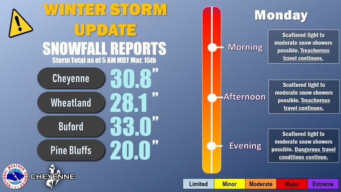
Cheyenne has seen 22.2” snow today. The 22.2” daily snowfall beats the old daily record of 19.8”, which was set on November 20, 1979. The 30.3” storm total surpasses the 25.6” that fell during November 19-21, 1979 to become Cheyenne’s biggest snowstorm on record.
-
Front Range snowstorm nowcast/conditions 3/13-15
donsutherland1 replied to mayjawintastawm's topic in Central/Western States
From the National Weather Service in Cheyenne: 818 CDUS45 KCYS 150333 CLICYS CLIMATE REPORT NATIONAL WEATHER SERVICE CHEYENNE WY 933 PM MDT SUN MAR 14 2021 ................................... ...THE CHEYENNE WYOMING AIRPORT CLIMATE SUMMARY FOR MARCH 14 2021... VALID TODAY AS OF 0900 PM LOCAL TIME. CLIMATE NORMAL PERIOD 1981 TO 2010 CLIMATE RECORD PERIOD 1871 TO 2021 WEATHER ITEM OBSERVED TIME RECORD YEAR NORMAL DEPARTURE LAST VALUE (LST) VALUE VALUE FROM YEAR NORMAL ................................................................... TEMPERATURE (F) TODAY MAXIMUM 31 144 AM 70 2003 47 -16 30 MINIMUM 23 759 PM -17 1880 24 -1 24 AVERAGE 27 36 -9 27 PRECIPITATION (IN) TODAY 1.91R 1.29 1946 0.03 1.88 0.01 MONTH TO DATE 2.61 0.41 2.20 0.42 SINCE MAR 1 2.61 0.41 2.20 0.42 SINCE JAN 1 3.33 1.21 2.12 1.21 SNOWFALL (IN) TODAY 22.2 R 11.5 1946 0.4 21.8 0.1 MONTH TO DATE 33.3 4.8 28.5 2.7 SINCE MAR 1 33.3 4.8 28.5 2.7 SINCE JUL 1 70.5 41.3 29.2 55.6 SNOW DEPTH 14 DEGREE DAYS HEATING TODAY 38 29 9 38 MONTH TO DATE 386 433 -47 375 SINCE MAR 1 386 433 -47 375 SINCE JUL 1 5304 5452 -148 5360 COOLING TODAY 0 0 0 0 MONTH TO DATE 0 0 0 0 SINCE MAR 1 0 0 0 0 SINCE JAN 1 0 0 0 0 ................................................................... WIND (MPH) HIGHEST WIND SPEED 36 HIGHEST WIND DIRECTION N (360) HIGHEST GUST SPEED 54 HIGHEST GUST DIRECTION N (350) AVERAGE WIND SPEED 23.3 SKY COVER POSSIBLE SUNSHINE MM AVERAGE SKY COVER 1.0 WEATHER CONDITIONS THE FOLLOWING WEATHER WAS RECORDED TODAY. THUNDERSTORM HEAVY SNOW SNOW LIGHT SNOW FOG FOG W/VISIBILITY <= 1/4 MILE RELATIVE HUMIDITY (PERCENT) HIGHEST 100 1200 AM LOWEST 88 1100 AM AVERAGE 94 .......................................................... THE CHEYENNE WYOMING AIRPORT CLIMATE NORMALS FOR TOMORROW NORMAL RECORD YEAR MAXIMUM TEMPERATURE (F) 48 76 2015 MINIMUM TEMPERATURE (F) 24 -13 1880 SUNRISE AND SUNSET MARCH 14 2021.........SUNRISE 712 AM MDT SUNSET 705 PM MDT MARCH 15 2021.........SUNRISE 710 AM MDT SUNSET 706 PM MDT - INDICATES NEGATIVE NUMBERS. R INDICATES RECORD WAS SET OR TIED. MM INDICATES DATA IS MISSING. T INDICATES TRACE AMOUNT. $$ The 22.2” daily snowfall beats the old daily record of 19.8”, which was set on November 20, 1979. The 30.3” storm total surpasses the 25.6” that fell during November 19-21, 1979 to become Cheyenne’s biggest snowstorm on record.