
bdgwx
-
Posts
1,520 -
Joined
-
Last visited
Content Type
Profiles
Blogs
Forums
American Weather
Media Demo
Store
Gallery
Everything posted by bdgwx
-
Copernicus won't publish the official numbers from ERA5 for another couple days. However, based on Hausfather's twitter post we might expect GISTEMP to publish around 1.10 C for June. ERA5 correlates with GISTEMP at R^2 = 0.89. Note that the previous record was 0.92 C in 2022. It is all but guaranteed at this point that June 2023 will be a new record in the GISTEMP dataset as well.
-
For the first time in recorded history the global average temperature breached 17 C; at least according to CFSR anyway.
-
I was actually getting ready to post the GFS forecast as well. You scooped me. Anyway, yeah, July is already forecasted to start off quite warm. I noticed that there was a small blip down in the global SST last week. I wonder if that means excess heat is transferring from the ocean into the atmosphere now. As of this moment my June expectation is a tick up to 1.08 ± 0.10. Once the June data starts rolling in I can get that uncertainty envelop down to ± 0.06 prior to the GISTEMP update. By all indications June 2023 is going to be the warmest June on record.
-
BTW...the page is buried pretty well. But you can get the probability density function corrected forecast (bias corrected) for the CFS from the following link. It took me forever to find it a couple of weeks ago and Google isn't much help. https://www.cpc.ncep.noaa.gov/products/people/wwang/cfsv2fcst/CFSv2SST8210.html
-
And the bias corrected CFS forecast is even lower at maybe +1.4.
-
I cannot disagree. If I have understood the Brown & Caldeira method correctly they only make predictions based on the current state of the climate system. In other words they do not take into account the expectation of future ENSO (or other highly correlated climatic element) states. This may explain why I get higher odds of a new record. My model is simpler (more like a multiple regression that minimizes RMSE), but incorporates the future expectation of ENSO and to a lesser extent total solar irradiance (which I do find to be at least minimally correlated with global temperatures). Both of which can be predicted 6 months in advance with reasonable skill. And yes, your point about global SST is well taken. My expectation is that the atmosphere will catch up to the higher SSTs in the next couple of months. It may be interesting to note that my model does not use SST has an input right now. In that regard one might argue that even I may be underestimating the warming potential in the later half of the year, but I'm going to remain more guarded on that matter as I also think a reversion to the trend may also be on the horizon. Afterall highly deviant increases/decreases tend to reverse some eventually. BTW...my current June expectation for GISTEMP is 1.07 ± 0.10 C. To put that into perspective even taking the ~2.5% chance that it comes in -0.10 C below the expectation at 0.97 C it will still easily surpass the previous record of 0.92 C set all the back in 2022. That should raise some eyebrows.
-
Brown & Caldeira are now saying there is a 57% chance of new GISTEMP record.
-
Berkeley Earth says there is a 54% chance of new record in their dataset.
-
@GaWx I bet you're right. I've not been able to find any daily ERSST updates. And I can't disagree, I see a very high correlation between NCEP/NCAR vs ERSST in ENSO 3.4 region at R^2 = 0.98. So while they don't match exactly it is very close. I certainly wouldn't dismiss it.
-
Someone can correct me if I'm wrong but it is my understanding that CDAS, which stands for Climate Data Assimilation System, is actually the model core for the NCEP/NCAR reanalysis. Or at least that is what the NCEP/NCAR built upon. The NCEP/NCAR reanalysis is known to be subpar. But I don't think that is justification for dismissing it outright. I do wonder if it wouldn't be better for Levi Cowan to use a more accepted product like OISST or ERSST though.
-
Several months back I suggested that if the shenanigans kept up in the Antarctic then perhaps it might be time for a dedicated thread. The data collected by the IPCC suggested that sea ice extents may increase through 2030 at the very least. Yet here we are with record lows. Perhaps the time for a dedicated thread as come.
-
Here is my latest expectation for GISTEMP which includes the June IRI ENSO ensemble forecast. Jan: 0.87 ± 0.01 C (3m lagged ENSO -0.99) Feb: 0.98 ± 0.01 C (3m lagged ENSO -0.90) Mar: 1.21 ± 0.01 C (3m lagged ENSO -0.86) Apr: 1.00 ± 0.01 C (3m lagged ENSO -0.71) May: 0.94 ± 0.02 C (3m lagged ENSO -0.46) Jun: 1.05 ± 0.12 C (3m lagged ENSO -0.11) Jul: 1.03 ± 0.22 C (3m lagged ENSO +0.13) Aug: 1.06 ± 0.23 C (3m lagged ENSO +0.39) Sep: 1.10 ± 0.24 C Oct: 1.13 ± 0.25 C Nov: 1.16 ± 0.26 C Dec: 1.17 ± 0.26 C 2023 Average: 1.06 ± 0.08 with 75% chance of a new record (>= 1.03)
-
The June IRI ensemble suite just got published. The statistical+dynamical average peak jumped up 0.2 to 1.5 on this update. https://iri.columbia.edu/our-expertise/climate/forecasts/enso/current/?enso_tab=enso-sst_table IRI June Seasons (2023 – 2024) Model JJA JAS ASO SON OND NDJ DJF JFM FMA Dynamical 1.295 1.539 1.679 1.761 1.746 1.598 1.473 1.264 1.009 Statistical 0.749 0.785 0.825 0.840 0.846 0.812 0.734 0.579 0.415 All 1.120 1.298 1.406 1.466 1.403 1.248 1.125 0.899 0.670
-
The bias corrected CFS peak has come down about 0.5 in the last few weeks.
-
This is great. I've been looking for an updated volcanic aerosol dataset for awhile now. I had no idea this existed. They even have it in an easy csv file format and it goes through 2022. Anyway, it looks like H2O adds about 0.1 W/m2 to the imbalance. Like you said the AOD portion is fading rapidly though so if the H2O portion is long term like scientists are expecting then we should expect a net positive, albeit small, effect from Hunga Tonga soon. Somewhat interesting...my machine learning model said a 5 month lag with GISTEMP for this volcanic aerosol dataset was optimal. My model was showing a -0.05 C adder to start the year and wanes to -0.02 C by the end after I extrapolate out the AOD decay based on what happened with Pinatubo.
-
ERA has a pretty high correlation with the traditional datasets. It correlates with GISTEMP at R^2 = 0.89. It's the same as JRA. The previous record via JRA was +0.34 (1991-2020 baseline) in 2019. So far the 2023 June value is +0.61. JRA correlation with GISTEMP is R^2 = 0.89 https://climatlas.com/temperature/jra55_temperature.php Similarly with the GFS as well. The previous record via GFS was +0.55 (1981-2010 baseline) in 2019. So far in 2023 June value is 0.68. GFS correlation with GISTEMP is R^2 = 0.78 http://www.karstenhaustein.com/climate.php
-
The May GISTEMP value came in at 0.94 C. This was a massive deviation and miss from my 1.05 ± 0.08 C expectation. A miss of that magnitude does not happen very often. And because May came in so much lower than my expectation my current June expectation drops to 1.06 ± 0.15 C. However, the Jan, Feb, and Mar values all came in 0.01 C higher so instead of dropping 0.11 from the yearly sum we only dropped 0.08 so the impact on the yearly average isn't as much as one might naively think. My current expectation for the full year average is now 1.05 ± 0.09 resulting in a probability of a new record (>= 1.03 C) of 67%. I should note that Nick Stokes' TempLS dataset has a very high correlation with GISTEMP (R^2 = 0.97) and gets released several days prior to GISTEMP. His dataset was suggesting the May anomaly would come in at 0.96 ± 0.06 C. As of the time of my 1.05 ± 0.08 C expectation I was not exploiting Nick's data. I will do so going forward.
-
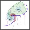
Relevant...
-
I'm skeptical of the Hunga Tonga effect myself. I've been tracking stratospheric temperature anomalies since the eruption and while there were very noticeable effects for about 8 months I can no longer see much of an effect. That's not to say that I don't think it will cause some warming, but I think it will be low enough that it will be indistinguishable from the noise. I do think there is merit to the marine aerosol reduction though. Even a tenth of watt change in the Earth energy imbalance (EEI) would be significant. Many of the marine emission rules went into effect in 2020 so it quite possible that at least some of the record setting temperatures can be traced back to the high EEI. If you look at @chubbs post above you'll see the CERES EEI is now +1.5 W/m2. CERES EEI calculations are known to have high uncertainty [Loeb et al. 2021], but +1.5 W/m2 is still high enough to raise eyebrows. There's no doubt that the main contribution of the higher 2023 temperatures is GHGs though. I think what is catching some off guard (like myself) is that the temperatures are higher than our expectations given that the 4 month lagged ONI corresponding to May was -0.7...well into La Nina territory. In other words, we're still under the La Nina influence albeit transitioning out now. Is it transient variation or is the warming really accelerating? One other significant contributing factor to the North Atlantic SSTs are believed to be high due to very low Saharan dust levels.
-
I hear what you saying. I take more of conservative position myself, but I will say that Hansen et al. 2022 indict the scientific community and especially the IPCC of "gradualism" so you've got support from others regarding your position. And we're talking about big names like Hansen, Schuckmann, Loeb, etc. who made this indictment.
-
The current data is interesting to say the least. I've been tracking both the record setting daily SST and daily 2mT. I'm not sure what to think of this. These are such extreme anomalies that they are statistically unlikely to persist even in a warming world so it makes me think they are transient and there will be a reversion to the trend soon. I have my model updated to better predict near term GISTEMP values. My May GISTEMP expectation is still 1.05 C, but with a much reduced uncertainty of ±0.08 C. And even though the May update isn't even published yet I'm already starting to see a big jump up in the June expectation given the current data. I'm going to go with 1.10 ± 0.16 C for June. And that could be low if temperatures don't come down from the first 1/3 of the month. I'm not going to post the monthly breakdown until the May GISTEMP and June IRI ENSO forecast are published, but a sneak peak of the final 2023 expectation does get bumped up to 1.07 ± 0.09 which puts the odds of a new record at 78%.
-
Yeah, that spike is running nearly 4σ above the 1981-2010 average and over 1σ above the previous record from all the way back in 2022 (via OISST). I'm not sure how this will effect the evolution of the current ENSO cycle or how it will affect the global scale circulation patterns. I do think a lot of this spike is occurring outside the tropical region, but at a cursory glance it appears there is enough contribution in the tropical region that it may attenuate the RONI values more than it might have otherwise.
-
Yep. I just setup my account today. I'll probably engage next week. Obviously I think the market is undervalued. I just updated my model with the latest data a few minutes ago. Below are my current expectations with 2σ confidence intervals. This averages out to 1.05 C. I'm estimating the uncertainty on the average at about ±0.09 C right now. That puts the probability of >= 1.03 at about 67%. My hunch tells me that is high. But past experience also tells me that hunches are terrible predictors so I don't know. Interestingly I don't actually have my model setup to optimally predict GISTEMP right now. I have it setup in a non-autocorrelated mode because I use it primarily to help explain the long term trend and short term variability; not to actually make informed near term predictions. I'll see if I can get it better tuned for 6 month lead time predictions. I also need to get the GISTEMP source code running on my machine again. I was actually running it a few years ago when I participated in another prediction market. I can use it to drive down the current month prediction uncertainty if I can get the daily ERSST and GHCN-M files incorporated into it. Note #1. The June uncertainty is still high because only 1 week of data is in. The uncertainty improves throughout the month. Note #2. My model has been low biased the first 4 months of the year so far. Note #3. I usually list the last few reported months as ±0.01-0.02 C because some observations are delayed by a few months getting into the repositories. Older months can change as well. It's just not as likely as the last few months. Jan: 0.86 ± 0.00 C Feb: 0.97 ± 0.01 C Mar: 1.20 ± 0.01 C Apr: 1.00 ± 0.02 C May: 1.05 ± 0.18 C Jun: 1.03 ± 0.22 C Jul: 1.02 ± 0.23 C Aug: 1.04 ± 0.24 C Sep: 1.07 ± 0.26 C Oct: 1.10 ± 0.26 C Nov: 1.12 ± 0.26 C Dec: 1.13 ± 0.26 C 2023 Average: 1.05 ± 0.09 with 67% chance of a new record (>= 1.03)
-
With the onset of El Nino and the possibility that 2023 could be a new record in some datasets I thought it might be nice to start a thread dedicated to the 2023 global average temperature. As of this posting the Kalshi prediction market for a new record according to GISTEMP is trading at $0.31. https://kalshi.com/markets/gtemp/global-average-temperature-deviation The Brown & Caldiera 2020 method is showing about a 50% probability of a new record for 2023 with a 76% chance of such for 2024. https://www.weatherclimatehumansystems.org/global-temperature-forecast My own machine learning model is saying there is about a 50% chance as well so this could be close.
-
So far the dynamic models are beating out the statistical models in terms of skill. As I understand that is typical through the spring forecast barrier, but once June comes around the statistical models start exhibiting similar skill to their dynamic counterparts. I wonder if we are going to see a jump up in the statistical average on the June IRI update?