
Jns2183
-
Posts
5,851 -
Joined
-
Last visited
Content Type
Profiles
Blogs
Forums
American Weather
Media Demo
Store
Gallery
Everything posted by Jns2183
-
Central PA Summer 2026 Discussion/Obs Thread
Jns2183 replied to Voyager's topic in Upstate New York/Pennsylvania
It goes in and out Sent from my SM-S731U using Tapatalk -
Central PA Summer 2026 Discussion/Obs Thread
Jns2183 replied to Voyager's topic in Upstate New York/Pennsylvania
Those first 4 days July is going to burn out the grass here and send us into not good drought conditions. For whatever reason @canderson and I have missed most of the rain this month. I sit at 1.25". We are in not good shape here and have been muddling along due to cool temperatures. That's all about io change and my soil moisture sensor already is at lowest ever 35%. Sent from my SM-S731U using Tapatalk -
Central PA Summer 2026 Discussion/Obs Thread
Jns2183 replied to Voyager's topic in Upstate New York/Pennsylvania
.08" puts me at 1.31" for June and 15.14" YTD. 4.53" below normal and good for 11th driest out of 131 years. Sent from my SM-S731U using Tapatalk -
Central PA Summer 2026 Discussion/Obs Thread
Jns2183 replied to Voyager's topic in Upstate New York/Pennsylvania
Some light reading Sent from my SM-S731U using Tapatalk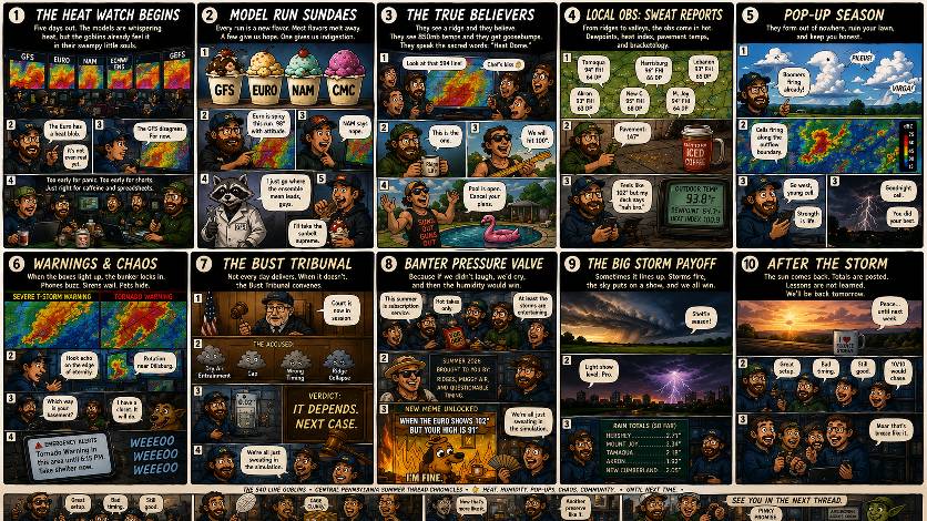
-
Central PA Summer 2026 Discussion/Obs Thread
Jns2183 replied to Voyager's topic in Upstate New York/Pennsylvania
Watching the Great outdoors I am one with the racoons Sent from my SM-S731U using Tapatalk
-
Central PA Summer 2026 Discussion/Obs Thread
Jns2183 replied to Voyager's topic in Upstate New York/Pennsylvania
Is there some aspect of it that you were looking for mostly I could probably guide you even further Sent from my SM-S731U using Tapatalk -
Central PA Summer 2026 Discussion/Obs Thread
Jns2183 replied to Voyager's topic in Upstate New York/Pennsylvania
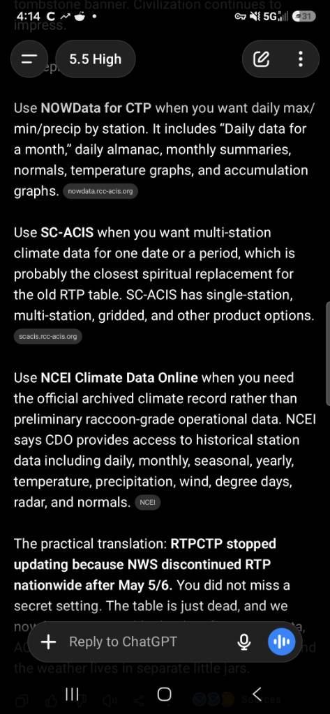
It's because they took it out to the wood shed and discontinued the product https://www.weather.gov/media/notification/pdf_2026/scn26-34_AR_ER_WR_RTP_Discontinuation.pdf The screenshot there has your best chances to find a replacement Sent from my SM-S731U using Tapatalk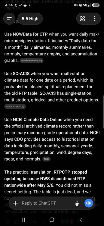
-
Central PA Summer 2026 Discussion/Obs Thread
Jns2183 replied to Voyager's topic in Upstate New York/Pennsylvania
What happened yesterday that my weather station only recorded .21" of rain Sent from my SM-S731U using Tapatalk -
Central PA Summer 2026 Discussion/Obs Thread
Jns2183 replied to Voyager's topic in Upstate New York/Pennsylvania
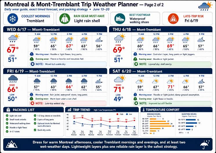
Heading up today to Montreal and Mont Tremblant, to apparently experience the April we never had here. And actually have to be faster days I will take that in the heart beat. After playing around with a bunch of different styles I think I've settled on this one for the perfect style for vacation weather sending out to everyone in the extended family who's going up there. Sent from my SM-S731U using Tapatalk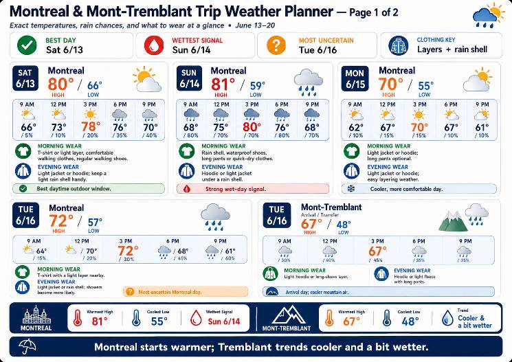
-
Central PA Summer 2026 Discussion/Obs Thread
Jns2183 replied to Voyager's topic in Upstate New York/Pennsylvania
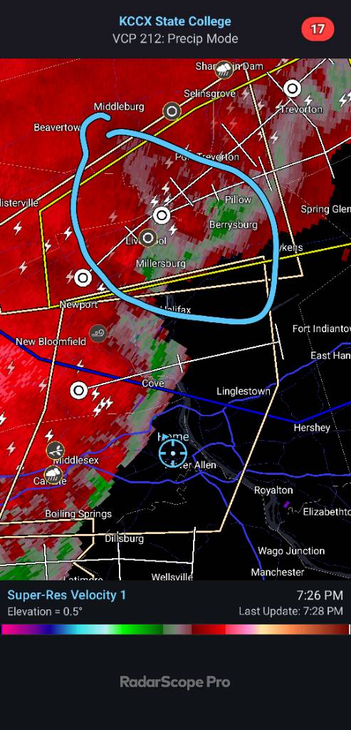
It seemed like all the storms yesterday at issues reading inflow from the rain core and essentially would choke themselves while the area around them played roulette with who is going to get to convergence from the competing outflow boundaries and who was going to get left in the dust. If you look at what happens when the storms congeal consolidate into a cold pool that cold pool axis pretty much a shovel throwing up all the warm moist air quickly upwards and technically that is what propagating it they original storms pretty much blow up die off while the cold pool constantly is pushing the warm moisture ahead giving the illusion of the storms actually moving. Yeah there is definitely a gradient to all this. Sent from my SM-S731U using Tapatalk -
Central PA Summer 2026 Discussion/Obs Thread
Jns2183 replied to Voyager's topic in Upstate New York/Pennsylvania
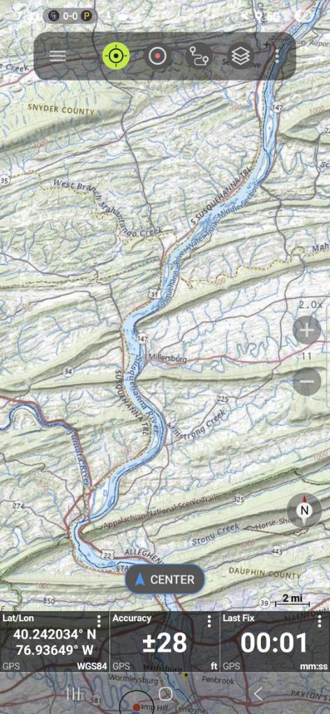
You sir have one the most studied watersheds in the nation with 5 minute data going back to 1968 Sent from my SM-S731U using Tapatalk -
Central PA Summer 2026 Discussion/Obs Thread
Jns2183 replied to Voyager's topic in Upstate New York/Pennsylvania
I currently sit at 13.89" for the year. Just about the 11th percentile If you folks want the most accurate rainfall history out there for your own backyard go here https://prism.oregonstate.edu/explorer/ 800m resolution and daily totals going back 1981 with monthly totals going back to 1895 Sent from my SM-S731U using Tapatalk -
Central PA Summer 2026 Discussion/Obs Thread
Jns2183 replied to Voyager's topic in Upstate New York/Pennsylvania
This a painful miss. Going to converge just east of river Sent from my SM-S731U using Tapatalk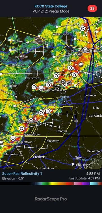
-
Central PA Spring 2026 Discussion/Obs Thread
Jns2183 replied to Voyager's topic in Upstate New York/Pennsylvania
Groundwater is a different animal to all of those things. You need to ask yourself what you are measuring because your measuring different things. There's things like river gauge level for things you want to measure. Sent from my SM-S731U using Tapatalk -
Central PA Spring 2026 Discussion/Obs Thread
Jns2183 replied to Voyager's topic in Upstate New York/Pennsylvania
Yup had entrainment and a cold pool while us in the valley got double teamed with cold pool and outflow flowing in from north and south. Future reminder is that if storms fire on both sides of the elevator train north and south of me to not expect much it's physics usually wins in the situations with cold air draining in undercutting all of our instability Sent from my SM-S731U using Tapatalk -
Central PA Spring 2026 Discussion/Obs Thread
Jns2183 replied to Voyager's topic in Upstate New York/Pennsylvania
.02". This area continues it's struggles when lots of others cash in. It's funny looking at 60 month maps and seeing a bullseye Sent from my SM-S731U using Tapatalk -
Central PA Spring 2026 Discussion/Obs Thread
Jns2183 replied to Voyager's topic in Upstate New York/Pennsylvania
Haha, it might be because people are still below the 40th percentile for ytd rainfall. Honestly unless we get area wide coverage of 25" from now till end of August I'd expect this map will be there the entire summer. Add in the fact that many have not had an above normal season in 3-4 years I'd be more worried if the map showed nothing. Sent from my SM-S731U using Tapatalk -
Central PA Spring 2026 Discussion/Obs Thread
Jns2183 replied to Voyager's topic in Upstate New York/Pennsylvania
Yum. I just made a beignet rum in our rotovap Sent from my SM-S731U using Tapatalk -
Central PA Spring 2026 Discussion/Obs Thread
Jns2183 replied to Voyager's topic in Upstate New York/Pennsylvania
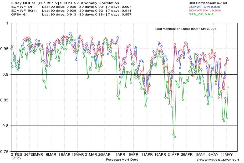
Tomorrow is apparently euro upgrade day and this new upgrade supposedly treats the GFS like used toilet paper. Sent from my SM-S731U using Tapatalk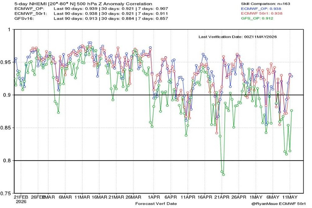
-
Central PA Spring 2026 Discussion/Obs Thread
Jns2183 replied to Voyager's topic in Upstate New York/Pennsylvania
Hoping for a reverse of last year. By end of May last year I was at 17.81" which is the 67th percentile yet I still finished in the 39th percentile for the year. I'm hoping for at least one good tropical influence storm this year hopefully 2. I'd love to get a good 20-25 inches of rain throughout the summer Sent from my SM-S731U using Tapatalk -
Central PA Spring 2026 Discussion/Obs Thread
Jns2183 replied to Voyager's topic in Upstate New York/Pennsylvania
I'm guessing 73 for. Memorial day Sent from my SM-S731U using Tapatalk -
Central PA Spring 2026 Discussion/Obs Thread
Jns2183 replied to Voyager's topic in Upstate New York/Pennsylvania
I sit at a dismal 9.74" of rain for the year which puts me at about the 21st percentile Sent from my SM-S731U using Tapatalk -
Central PA Spring 2026 Discussion/Obs Thread
Jns2183 replied to Voyager's topic in Upstate New York/Pennsylvania
So here is a fun little project. It's CTP entire event database since 1996. Tried to normalize reports by population and homogenize costs to compare. You can do a neat little heatmap that shows preferred storm corridors to some extent. You definitely can't totally escape the rule that someone has to be there to make a storm report, but I did try to balance it out. I think there's almost 10,000 events. You can filter by all kinds of things. Enjoy!!! https://jns182wx.github.io/CTP_Storm_Catalog/ Sent from my SM-S731U using Tapatalk -
Central PA Spring 2026 Discussion/Obs Thread
Jns2183 replied to Voyager's topic in Upstate New York/Pennsylvania
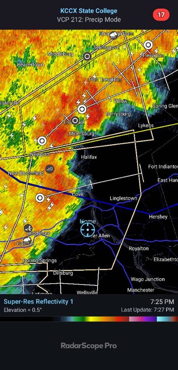
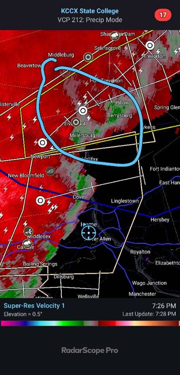
Yes, it's broad but I swear I see more rotation in lines consistently than any other spot right in this area where the mountains form a V that I wonder if its terrain enhanced Sent from my SM-S731U using Tapatalk -
Central PA Spring 2026 Discussion/Obs Thread
Jns2183 replied to Voyager's topic in Upstate New York/Pennsylvania
Yes, it's broad but I swear I see more rotation in lines consistently than any other spot right in this area where the mountains form a V that I wonder if its terrain enhanced Sent from my SM-S731U using Tapatalk